jsQuestPlus
Fitting and plotting the results
One useful feature that jsQuestPlus does not provide, but that QUEST+ based on Mathematica and MATLAB do, is fitting a psychometric function and plotting the results. Fitting allows estimation of psychometric parameters beyond the constraints of the quantized parameter space. Although the fitting or plotting functions cannot be performed during an online experiment, they can be performed afterwards using Mathematica or MATLAB.
This section explains how to use the MATLAB-based qpFit function to fit the jsQuestPlus data. Note that the qpFit function requires the Optimization Toolbox (The MathWorks, Inc.).
Save the stimulus paramters and responses.
For fitting, the stimulus parlameters and responses in all trials are needed. The method of saving the data depends on the experimental tool you are using. Please refer to the tool’s documentation for specific instructions.
For example, if you use jsPsych, you can save the data as follows:
on_finish(data){
    const response = jsPsych.pluginAPI.compareKeys(data.response, 'f') ? 1 : 0;
    jsqp.update(stim, response);

    // Save the stimulus and response data for the MATLAB-based qpFit program.
    data.stim = stim;
    data.outcome = response + 1; // The responses in JavaScript is 0 or 1, but in MATLAB these correspond to 1 or 2.
}
We have a demo which outputs a CSV file.
Arrange the data
Here is the MATLAB code to import the file and arrange the data. Note that the first and last rows in the sample CSV file are not needed.
trialDataTable = readtable("mydata.csv");
trialDataTable([1,end],:) = []; % Delete unnecessary rows.
trialData = table2struct(trialDataTable(:,{'stim', 'outcome'})); % Extract necessary columns and convert it to structure array.
Fitting the results
We refer to qpQuestPlusCoreFunctionDemo.m
psiParamsQuest = [-20, 3.5, 0.5, 0.02]; % jsqp.getEstimates() returns the values at the end of the series of trials.
nOutcomes = 2;

%% Find aximum likelihood fit.  Use psiParams from QUEST+ as the starting
% parameter for the search, and impose as parameter bounds the range
% provided to QUEST+.
psiParamsFit = qpFit( ...
    trialData, ... % results from online experiments
    @qpPFWeibull, ...
    psiParamsQuest, ... % estimates from online experiments
    nOutcomes, 'lowerBounds', [-40 2 0.5 0],'upperBounds',[0 5 0.5 0.04]);

fprintf('Maximum likelihood fit parameters: %0.1f, %0.1f, %0.1f, %0.2f\n', ...
    psiParamsFit(1),psiParamsFit(2),psiParamsFit(3),psiParamsFit(4));
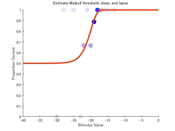
Plotting the results
We refer to qpQuestPlusCoreFunctionDemo.m
%% Plot of trial locations with maximum likelihood fit
figure; clf; hold on
stimCounts = qpCounts(qpData(trialData),nOutcomes);
stim = [stimCounts.stim];
stimFine = linspace(-40,0,100)';
plotProportionsFit = qpPFWeibull(stimFine,psiParamsFit);
for cc = 1:length(stimCounts)
    nTrials(cc) = sum(stimCounts(cc).outcomeCounts);
    pCorrect(cc) = stimCounts(cc).outcomeCounts(2)/nTrials(cc);
end
for cc = 1:length(stimCounts)
    h = scatter(stim(cc),pCorrect(cc),100,'o','MarkerEdgeColor',[0 0 1],'MarkerFaceColor',[0 0 1],...
        'MarkerFaceAlpha',nTrials(cc)/max(nTrials),'MarkerEdgeAlpha',nTrials(cc)/max(nTrials));
end
plot(stimFine,plotProportionsFit(:,2),'-','Color',[1.0 0.2 0.0],'LineWidth',3);
xlabel('Stimulus Value');
ylabel('Proportion Correct');
xlim([-40 00]); ylim([0 1]);
title({'Estimate Weibull threshold, slope, and lapse', ''});
drawnow;
Sample image
You will get the following figure.